GWSDAT
GWSDAT Version 3.3 now released! Updates include:
- Easier Installation: GWSDAT's Excel deployment has been redesigned for easier and more robust installation which no longer requires administrative rights. See Installation Instructions here.
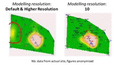
- Faster Spatiotemporal Modelling: The GWSDAT add-in now comes bundled with a portable Windows R version optimized for linear algebra which enables the spatiotemporal model to run quicker for higher resolution model settings. This enables users to more readily increase the modelling resolution which can be useful for fixing occurrences of the statistical anomaly referred to as 'ballooning'. For full details article here: https://doi.org/10.1002/env.2347
- GWSDAT Tutorials - YouTube: https://www.youtube.com/channel/UCtvo_J3B1hSPwKQxO9GqbWQ
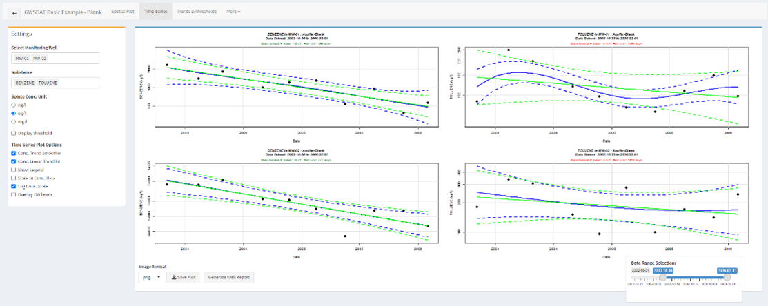
- Upgraded Well Time Series Plot:
- Functionality to specify time range of data in Well Time-Series plot.
- Functionality to select multiple wells and solutes for matrix style plots.
- New R package released on CRAN and GitHub. Full list of changes available.
Updated User Manual: http://gwsdat.net/gwsdat_manual
Bug Fixes and Enhancements:
- Functionality to export spatial plot predictions to ASCII file format.
- Functionality to aggregate temporal plotting resolution to Semi Annual.
- CSS styling for Trends and Thresholds plot which includes scrolling for many wells and solutes.
- Functionality to Select/Deselect all wells in reports and predictions.
GWSDAT is an open source, user-friendly software application for the visualisation and interpretation of groundwater monitoring data.
Key functionalities:
- Trend analyses
- Data smoothing
- Spatiotemporal smoothing
- Determination of contamination plume characteristics
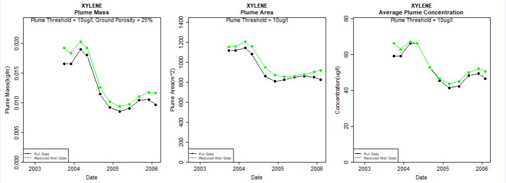
- Well redundancy analysis
- Automatic report generation tools
Business Benefits:
- Early identification of increasing trends or off-site migration.
- Holistic evaluation of groundwater trends.
- Nonparametric statistical and uncertainty analyses.
- Reduction in long-term monitoring sites.
- Efficient reporting via standardised plots and tables.
- Well redundancy optimisation.
Introduction:
The GroundWater Spatiotemporal Data Analysis Tool (GWSDAT) has been developed by Shell Global Solutions for the analysis of groundwater monitoring data. It is designed to work with simple time-series data for solute concentration and ground water elevation, but can also plot non-aqueous phase liquid (NAPL) thickness if required. Spatial data is input in the form of well coordinates, and wells can be grouped to separate data from different aquifer units. The software also allows the import of a site basemap in GIS shapefile format. Concentration trend and 2D contour plots generated using GWSDAT can be exported directly to Microsoft PowerPoint and Word to expedite reporting.
Software Architecture:
The application is supported for Windows 8 and 10 and the corresponding version of Microsoft Office (including 64-bit operating systems). Data input to GWSDAT is via a standardized Excel spreadsheet and the data analysis and plot functions are accessed through an Excel Add-in application. The statistical engine used to perform geo-statistical modelling and display graphical output is the open- source statistical programming language R (www.r-project.org). A user manual and two example datasets are provided with the software for training and demonstration purposes.
The modelling of solute distribution in groundwater is typically restricted to either the analysis of trends in individual wells or independent fitting of spatial concentration distributions (e.g. by Kriging) to data from monitoring events. Neither of these techniques satisfactorily elucidate the interaction between spatial and temporal components of the data.
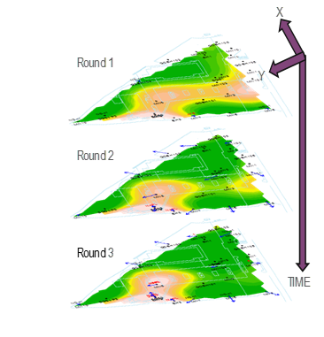
GWSDAT applies a spatiotemporal model smoother for a more coherent and smooth interpretation of the interaction in spatial and time-series components of groundwater solute concentrations. A spatiotemporal concentration smoother is fitted for each analyte using a non-parametric regression technique known as Penalised Splines (Eilers and Marx, 1992, 1996). A Bayesian methodology is used to select the appropriate degree of model smoothness (Evers et al, 2015).
The fit of the spatiotemporal algorithm to the monitoring data can be evaluated.
The GWSDAT graphical user interface (GUI) allows the user to navigate through a groundwater dataset and explore concentration/ groundwater elevation trends in individual wells and across the site. Several options are available to customize the display and data analysis. Note that plots can also be automatically exported.
-
GWSDAT includes the following tools for trend visualization and detection:
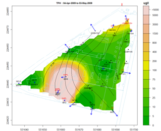
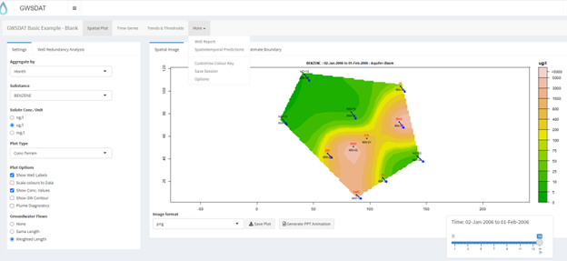
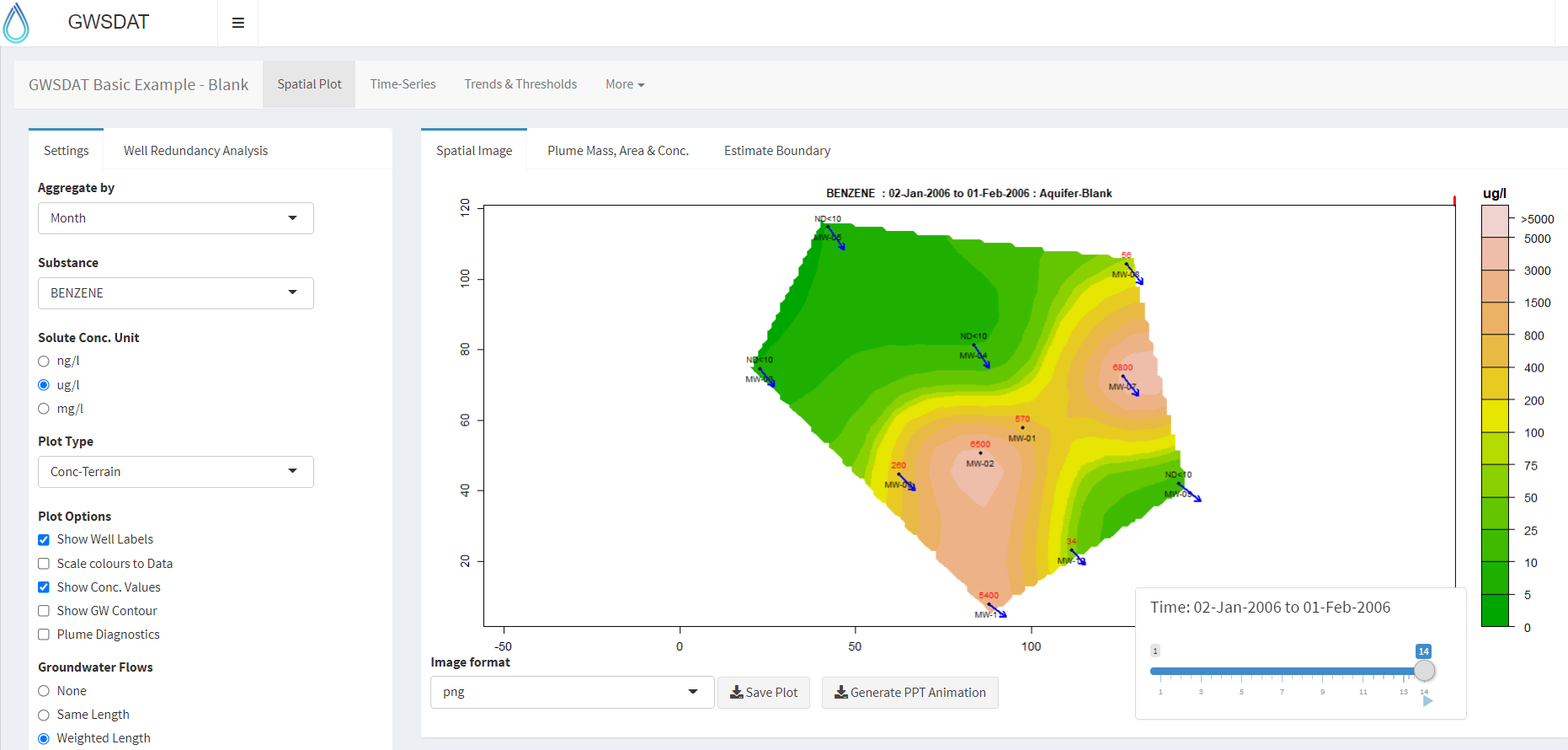
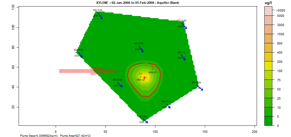
Spatial plot: For the analysis of spatial trends in solute concentrations, groundwater flow and, if present, NAPL thickness. Overlaid on this plot are the predictions of the spatiotemporal solute concentration smoother which is a function that simultaneously estimates both the spatial and time series trend in site solute concentrations. GIS shapefiles can also be overlaid on this plot.
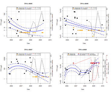
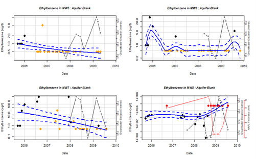
Well Trend plot: For the investigation of historical time-series trends in solute concentrations, groundwater elevation and, if present, NAPL thickness for individual wells. Users can overlay a nonparametric smoother which estimates the time-series trend in solute concentration. The advantage of this nonparametric method is that the trend estimate is not constrained to be monotonic, i.e. the trend can change direction.
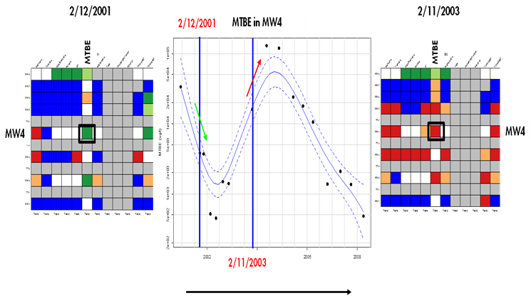
Trend and Threshold Indicator Matrix: This feature provides a summary of the level and time series trend in solute concentrations at a particular model output interval.
.
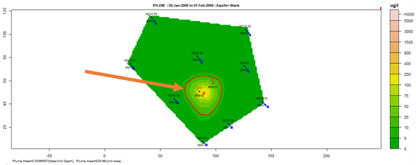
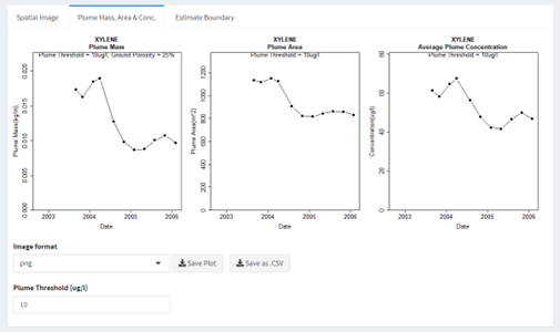
Plume diagnostics plots: This feature enables to calculate and display plume diagnostic quantities (area, mass, concentration) for a delineated plume displayed with a solid red contour line
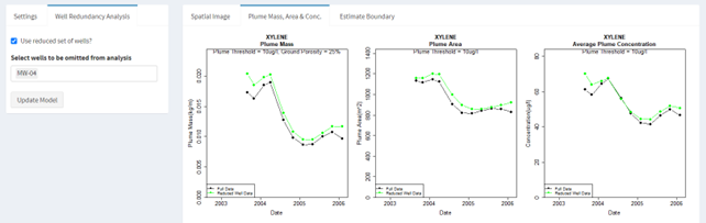
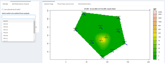
Well redundancy: This feature enables the user to very conveniently drop a well or a combination of wells from the analysis and investigate the resultant impact.

Well Influence Analysis: Building on the existing well redundancy analysis feature, GWSDAT now provides an ordered well omission list such that the wells estimated to have the least influence are presented first. This offers users more assistance in assessing which monitoring wells may be the most suitable for future omission and eventual decommissioning. This well influence order is established via a procedure fully documented here and here.
The GWSDAT V3.3 Excel Add-in has a new simpler installation procedure where all files are bundled together, and you don’t need admin rights to install the software. Before attempting installation, it is recommended to read the article here for more information on Excel Trusted Locations and add-in troubleshooting. A video demonstrating end to end installation can be found here.
Installation Instructions:
1) Download https://gwsdat.net/r-portable-win/ and unzip to an Excel Trusted Location on your C drive (not a network drive). e.g. C:\Users\User.Name\AppData\Local\GWSDAT\R-Portable-Win\R-Portable-Win\library. This may take a few minutes.
2) Open Excel and install the GWSDAT add-in by choosing: "File" > "Options" > "Add-Ins" > "Go" > "Browse" and then select "GWSDAT V3.3.xlam" located in the "C:\Users\User.Name\AppData\Local\GWSDAT\R-Portable-Win\R-Portable-Win\library\GWSDAT\extdata" folder. To avoid any Excel add-in security issues please ensure that this is a trusted location.
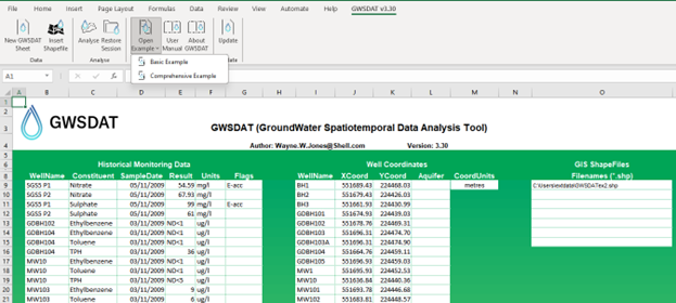
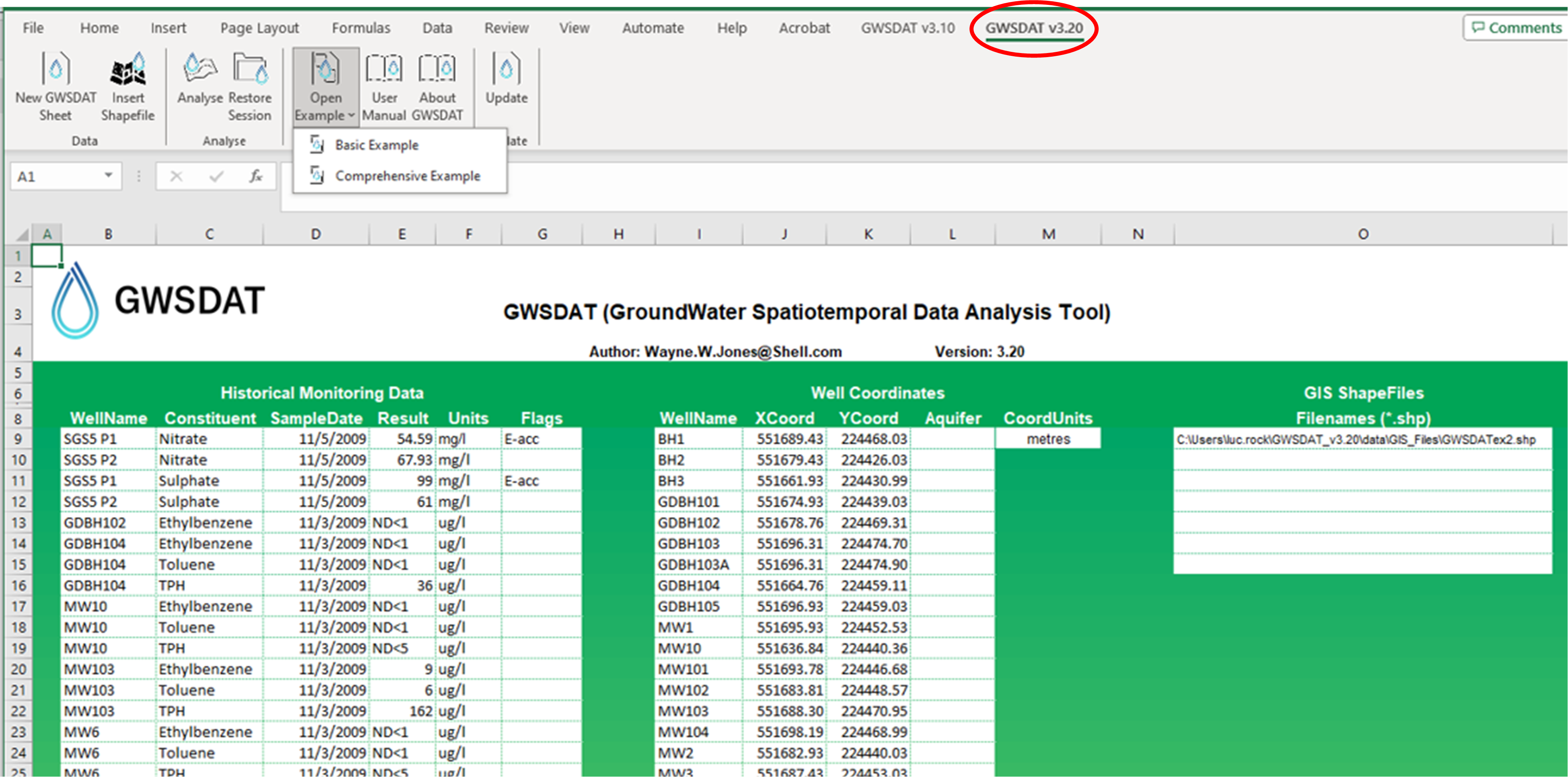
3) A menu called "GWSDAT v3.3" will appear in the EXCEL ribbon (on right side) along the top of the EXCEL window. To get started with a basic example activate menu by clicking on “GWSDAT v3.3”and then select “Open Example” - select “Basic Example" and then select "Analyse”.
Troubleshooting:
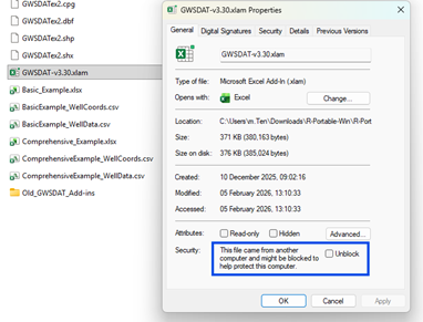
If the “GWSDAT v3.3” menu does not appear in Excel or an add-in error occurs, then follow the steps in this article here. Most commonly, the solution here is to unblock the add-in file.
Navigate to “C:\Users\User.Name\AppData\Local\GWSDAT\R-Portable-Win\R-Portable-Win\library\GWSDAT\extdata” folder and check the file “GWSDAT V3.3.xlam” isn’t blocked by doubling click on it. If it is blocked then right click the file, select properties and check the unblock check as seen in the screenshot below.
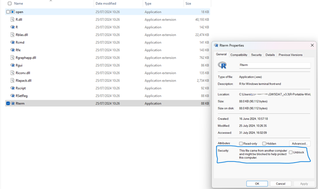
If the “GWSDAT v3.3” menu is visible, but nothing happens when you run the example then please navigate to “C:\Users\User.Name\AppData\Local\GWSDAT\R-Portable-Win\R-Portable-Win\bin\x64” and check the file “Rterm.exe” isn’t blocked. You can check it isn’t blocked by double clicking on the file. If it is blocked then right click the file, select properties and check the unblock check as seen in below screenshot
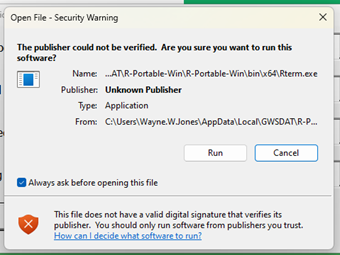
You may see a security warning – as screenshot below – click run to proceed and uncheck “Always ask before opening this file” to stop this message appearing in the future.
- ·To get started with a basic example activate menu by clicking on “GWSDAT v3.30”and then select “Open Example” ▶️select “Basic Example" and then select "Analyse”.
- Note- the first time you run this it may take a while as it needs to download and install some additional R packages.
- To get started with a more complex example activate menu by clicking on “GWSDAT v3.30”and then select “Open Example”▶️ select “Comprehensive Example”, and then select "Analyse”.
GWSDAT Data Entry
What types of monitoring data can be entered into GWSDAT?
Time series groundwater solute concentration (in ng/L, ug/L or mg/L units)
Time series groundwater elevation (relative to a common ordnance datum)
Time series NAPL thickness
Well coordinates (in Cartesian coordinates, not latitude, longitude)
I don’t have grid references for the groundwater monitoring wells, can I still use GWSDAT?
Yes, scalar X,Y well coordinates can be measured direct from a site plan. For example, by aligning a transparent grid of numbered squares with the N-S arrow on the site plan (north upwards) and reading off the relative X,Y locations of each well.
Can site plans be uploaded into GWSDAT?
Yes, site plans in GIS Shapefile format can be imported as background images. The filepath to the Shapefile folder is entered in the third table of the Excel data input worksheet (entitled “GIS ShapeFiles”). The user can either enter the shapefile location manually or use the `Browse for Shapefile' function in the GWSDAT Excel menu for interactive file selection. Only the location of the main shapefile (file ending with a `.shp' extension) needs to be specifed in this table - the associated data files (e.g. .dbf, .sbn, .sbx, .shx) will be picked up automatically, provided they are in the same folder. It is possible to overlay multiple shapefiles up to a maximum of seven. Please refer to the GWSDAT user manual for additional information, including the conversion of CAD drawing layers to Shapefile format using ARC-GIS.
Can depth- dependent (e.g. multilevel) groundwater data be visualised using GWSDAT?
No, it is not possible to model vertical concentration distribution using GWSDAT. However, it is possible to group monitoring wells (e.g. by aquifer) and then plot each group separately. Multiple concentration values for a given solute at the same X,Y location, well group and sampling time are detected by GWSDAT and averaged prior to fitting of the spatiotemporal model.
In the event that a site- wide 3D interpretation of groundwater flow and solute transport is required we would recommended the use of numerical modelling software such as FEFLOW or MODFLOW. The considerable time and effort required to populate and run such complex models may be justified for high profile sites when working with high- cost 3 dimensional aquifer data.
What are the minimum input data requirements for GWSDAT to function correctly?
The minimum input data requirements for GWSDAT to run correctly are as follows: For plotting of groundwater flow direction arrows:
- No solute concentration data required
- Minimum 3 well locations in coordinate table
- Minimum 1 measurement of groundwater elevation at each of these 3 wells within the user- selected model output interval
For plotting of groundwater elevation contours:
- No solute concentration data required
- Minimum 4 well locations in coordinate table
- Minimum 1 measurement of groundwater elevation at each of these 4 well locations within the user- selected model output interval
For plotting of solute concentration trends at individual wells:
- Minimum one solute: No groundwater elevation data required
- Minimum 1 well location in coordinate table
- Minimum 1 measurement of groundwater solute concentration at this well location
For fitting of valid spatiotemporal model and plotting of solute concentration contours:
- Minimum one solute: No groundwater elevation data required
- Minimum 3 well locations in coordinate table
- Minimum 2 concentration, time data points for each of these 3 well coordinates
What are the minimum input data requirements for representative solute concentration contouring?
In order to generate representative concentration contour plots, the spacing of monitoring wells needs to reflect the characteristic distance over which solute concentrations vary in the groundwater. This will vary from site to site: if groundwater flow rates are low or solute transport retarded then concentration hotspots are likely to occur and a closer well spacing will be required to map the concentration distribution. Conversely, if groundwater flow rates are high and solute transport is not significantly retarded then a larger well spacing may be adequate to map the concentration distribution.
Because the minimum well spacing required for effective concentration contouring varies from site to site, the user’s judgement is required in deciding whether the available data merits contouring. The presence of “redundant” data points that can be removed without significantly changing the concentration distribution is an indication that the monitoring well spacing is more than sufficient.
In the event that only a small number of wells (i.e. <4) are present, then GWSDAT v2.0 includes a circle plot option, which represents the data as circles coloured and sized to solute concentration, thereby avoiding the need to use potentially misleading concentration contours.
Similar arguments apply to the contouring of groundwater elevation data, although in the absence of significant topographic variation/ geological heterogeneity or groundwater abstraction/ water injection groundwater piezometric surfaces should be locally planar. The adaptive kriging algorithm used by GWSDAT to derive the piezometric surface requires a minimum of 4 well locations; flow direction arrows can, however, be generated for only 3 well locations.
How does the non- detect substitution function work?
GWSDAT handles non-detect data by a method of substitution. In accordance with general convention, the default option is to substitute the non-detect data with half its detection limit, e.g. ND<50ug/l is substituted with 25ug/l. Alternatively, non-detect data can be substituted with its full detection limit, e.g. ND<50ug/l is substituted with 50ug/l. Note that the entry of zero concentration values is not permitted.
How does the software handle Non Aqueous Phase Liquid (NAPL) data?
During data analysis the user has the option to ignore the presence of NAPL when fitting the spatiotemporal model, or substitute detections of NAPL with site maximum solute concentrations. NAPL substitution should only be used if it is known that the solutes entered into GWSDAT are derived from dissolution of the NAPL. This functionality was introduced to avoid the situation whereby an area of wells containing NAPL appears as a minimum on concentration contour plots because groundwater solute concentration data is not available.
Note: Any solutes that are not derived from the NAPL can be excluded from the NAPL substitution process by flagging them as “NotInNAPL” or “E-acc” in the historical monitoring data table of the input worksheet. Note also that only one solute data point needs to be flagged to remove that solute from the substitution algorithm.
GWSDAT Data Analysis/Plotting functions - Functions associated with spatial plot window
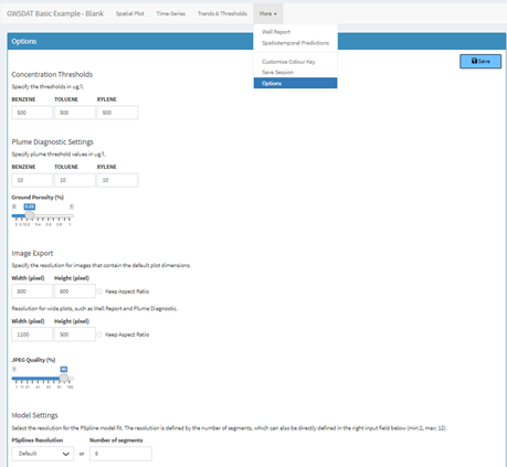
How can the model output interval be varied (i.e. time interval at which solute concentration/ NAPL thickness/ piezometric contours are reported)?
The “GWSDAT options” dialogue box, which appears when “GWSDAT analysis” is selected, allows the user to select the time interval between spatiotemporal model output plots. The pre-defined user options are “None”, “Monthly” or “Quarterly”: the model sets the start and end dates for the intervals by working backwards from the most recent sampling date. Concentration contour plots are generated by exporting data from the spatiotemporal model at the end of each specified time interval.
The “GWSDAT options” dialogue box also controls the handling of groundwater elevation data. If no aggregation (i.e. “None”) is selected then the software will attempt to generate a groundwater contour plan for every date in the input dataset. In practice, however, groundwater elevation surveys are often spread over a number of days and so this approach is likely to generate incomplete contour plots. If “monthly” or “quarterly” aggregation selected the software collates daily groundwater elevation data into monthly or quarterly blocks, thereby increasing the size of the dataset available for piezometric contouring.
How are solute concentration contours generated?
Solute concentration contours are generated using a spatiotemporal smoother algorithm, which fits a model to the solute concentration distribution through space (XY well coordinates) and time. This does not involve any temporal collation of the input concentration dataset. For further details refer to GWSDAT software manual.
How are groundwater piezometric contours generated?
Piezometric contours are generated using an adaptive kriging algorithm. The degree of flexibility allowed by the kriging algorithm is a function of the number of groundwater elevation data points in the selected model output interval, which improves the contour quality for smaller datasets.
How does the software scale the concentration contour/ circle plots?
Solute concentration contour plots have default logarithmic scales of 0 to >50,000 ng/L, 0 to >5000 ug/L or 0 to > 500 mg/L, dependent on the units selected. The concentration scale is fixed so that contour plots for successive time slices are directly comparable. The user can, however, select to “scale colours to data” to produce a colour key scaled to the concentration range for each model output interval.
GWSDAT Software Settings
The GWSDAT Graphical User Interface is bigger than my screen. How do I reduce the size?
This issue sometimes arises with low screen resolution. To modify the size of the GWSDAT Graphical User Interface you need to go in to the Excel VBA code module “ConfigParams” within “GWSDAT V2.0.xla” and change the following line of code:
(To access the VBA code –press Alt+F11 from Excel).
Change the code:
Public Const PanelScaling = 1 'Sizing of GWSDAT interface
To something like this:
Public Const PanelScaling = “0.75" 'Sizing of GWSDAT interface
When you are happy with the size of the GWSDAT user interface save the add-in by choosing File->Save GWSDAT V2.0.xla from the VBA editor.
Please see http://gwsdat.net/gwsdat_manual/ for comprehensive user manual and supporting material.
To report any software issues or bugs please fill in the user feedback form here: http://gwsdat.net/feedback/ .
Please note that CL:AIRE / Shell Global Solutions do not provide consultancy on data interpretation or use of the GWSDAT software.
Article: Groundwater Spatiotemporal Data Analysis Tool – Case Studies, New Features and Future Developments.
GWSDAT is listed in the following ITRC guidance document: Groundwater statistics for Monitoring and Compliance
Case studies: http://gwsdat.net/case-studies/
Article: Groundwater Spatiotemporal Data Analysis Tool: Case Studies, New Features and Future Developments
Article: on benefits of spatiotemporal modelling GWSDAT in Science of Total Environment.
Article: on GWSDAT in Science Direct
Article: "Analyzing Groundwater Quality Data and Contamination Plumes with GWSDAT" in Groundwater
Supporting information for the above Groundwater article:
The authors gratefully acknowledge those people who have contributed their knowledge and time to the development of GWSDAT.
The authors wish to express their gratitude to Adrian Bowman, Claire Miller, Craig Alexander, Craig Wilkie, Ludger Evers and Daniel Molinari from the department of Statistics, University of Glasgow, for their invaluable contributions to the development of the spatiotemporal algorithm.
Thanks also to Ewan Mercer from the University of Glasgow for his assistance in the development of the GWSDAT user interface.
We acknowledge and thank the R project for Statistical Computing and all its contributors without which this project would not have been possible.
A big thank you to Shell's worldwide environmental consultants for assistance in evaluating and testing the earlier versions of GWSDAT.
Thanks also to the Shell Year in Industry students who spent a great deal of time testing GWSDAT and making suggestions for improvements.
Thanks to Andrew Kirkman and team from BP Remediation Solutions for contributing new functionality and enhancements in version 3.3.
Thanks to Fraser Spalding who as a summer student at the University of Glasgow, almost singlehandedly, delivered the GWSDAT Tutorials YouTube Channel.
Credit and acknowledgement to Jan Limbeck from Shell for providing the portable Windows R version optimized for linear algebra.
We thank both current and former colleagues including Matthew Lahvis, Jonathan Smith, George Devaull, Dan Walsh, Curtis Stanley, Marco Giannitrapani and Philip Jonathan for their support, vision and advocacy of GWSDAT.
Bowman and Azzalini, 1997. Applied Smoothing Techniques for Data Analysis: the Kernel Approach with S-Plus Illustrations. Oxford University Press, Oxford, 1997.
Bowman and Azzalini. sm: Smoothing methods for nonparametric regression and density estimation. R package, www.stats.gla.ac.uk/~adrian/sm
Eilers and Marx, 1992. Generalized Linear Models with P-Splines in Advances in GLIM and Statistical Modelling (L.Fahrmeir et al.eds.). Springer, New York.
Eilers and Marx, 1996. Flexible smoothing with b-splines and penalties. Statistical Science 11, 89–121.
Evers et al., 2015. Efficient and automatic methods for flexible regression on spatiotemporal data, with applications to groundwater monitoring, Environmetrics (open access), 26(6), 431-441.
Jones, et al., 2014. A software tool for the spatiotemporal analysis and reporting of groundwater monitoring data (open access), Environmental Modelling and Software, 55, 242-249.
Jones, et al., 2015. Analyzing Groundwater Quality Data and Contamination Plumes with GWSDAT (open access), Groundwater, 53 (4), 513-514.
McLean et al., 2019, Statistical modelling of groundwater contamination monitoring data: A comparison of spatial and spatiotemporal methods, Science of The Total Environment (open access), 652, 1339-1346.
R Development Core Team. R: A Language and Environment for Statistical Computing. R Foundation for Statistical Computing, Vienna, Austria, 2-008. ISBN 3-900051-07-0, http://www.r-project.org
GWSDAT v3.2 now released!
Click here for a list of important updates.
What is GWSDAT?
GWSDAT is an open source, user-friendly, software application for the visualisation and interpretation of groundwater monitoring data. It also enables to work with other types of monitoring data collected over time and space (e.g. soil gas concentrations).
Key functionalities of tool:
- Trend analyses
- Data smoothing
- Spatiotemporal smoothing
- Determination of contamination plume characteristics
- Well redundancy analysis
- Automatic report generation tools based on user input.
Business Benefits
GWSDAT, through improved risk-based decision making and response, adds value in several different ways:
- Early identification of increasing trends or off-site migration.
- Evaluation of groundwater monitoring trends over time and space (i.e., holistic plume evaluation).
- Nonparametric statistical and uncertainty analyses to assess highly variable groundwater data.
- Reduction in the number of sites in long-term monitoring or active remediation through simple, visual demonstrations of groundwater data and trends.
- More efficient evaluation and reporting of groundwater monitoring trends via simple, standardised plots and tables created at the ‘click of a mouse.’
- Well Redundancy Analysis functionality to identify potential optimization measures with regards to monitoring well network sampling locations.
GWSDAT V3.2 updates
- Well Influence Analysis: Building on the existing well redundancy analysis feature, GWSDAT now provides an ordered well omission list such that the wells estimated to have the least influence are presented first. This offers users more assistance in assessing which monitoring wells may be the most suitable for future omission and eventual decommissioning. This well influence order is established via a procedure fully documented here and here.
- GW Well Report Functionality: Ability to export the full collection of Well Time Series plots which can include overlaid groundwater and NAPL thickness. See section 6.5 of the user manual – here.
- For GWSDAT R Developers:
- New R package released on CRAN here and on GitHub here.
- New functionality to read in data.frames directly to the GWSDAT R package – see here.
- Beta implementation of online GWSDAT Application Programming Interface (API). This allows users to pass data directly to the online version via URL arguments - see here.
- Updated User Manual: http://gwsdat.net/gwsdat_manual. A fully comprehensive updated description of GWSDAT - including Well Influence Analysis.
- Bug Fixes and Enhancements: Numerous bug fixes and enhancements. For example, support for Windows Meta File image format output for spatial plot - useful for rearranging overlapping well labels. Updated Excel Add-in - more robust to 32 bit versus 64 bit version of Excel.
Background
Introduction
The GroundWater Spatiotemporal Data Analysis Tool (GWSDAT) has been developed by Shell Global Solutions for the analysis of groundwater monitoring data. It is designed to work with simple time-series data for solute concentration and ground water elevation, but can also plot non-aqueous phase liquid (NAPL) thickness if required.
Spatial data is input in the form of well coordinates, and wells can be grouped to separate data from different aquifer units. The software also allows the import of a site basemap in GIS shapefile format. Concentration trend and 2D contour plots generated using GWSDAT can be exported directly to Microsoft PowerPoint and Word to expedite reporting.
Software Architecture
The application is supported for Windows 8 & 10 and the corresponding version of Microsoft Office (including 64-bit operating systems). Data input to GWSDAT is via a standardized Excel spreadsheet and the data analysis and plot functions are accessed through an Excel Add-in application.
The statistical engine used to perform geo-statistical modelling and display graphical output is the open- source statistical programming language R (www.r-project.org). A user manual and two example datasets are provided with the software for training and demonstration purposes.

{multithumb}
Spatiotemporal Data Analysis
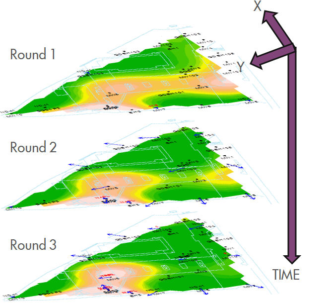 The modelling of solute distribution in groundwater is typically restricted to either the analysis of trends in individual wells or independent fitting of spatial concentration distributions (e.g. by Kriging) to data from monitoring events. Neither of these techniques satisfactorily elucidate the interaction between spatial and temporal components of the data.
GWSDAT applies a spatiotemporal model smoother for a more coherent and smooth interpretation of the interaction in spatial and time-series components of groundwater solute concentrations. A spatiotemporal concentration smoother is fitted for each analyte using a non-parametric regression technique known as Penalised Splines (Eilers and Marx, 1992, 1996).
A Bayesian methodology is used to select the appropriate degree of model smoothness (Evers et al, 2015). The fit of the spatiotemporal algorithm to the monitoring data can be evaluated.
Graphical User Interface
 The GWSDAT graphical user interface (GUI) allows the user to navigate through a groundwater dataset and explore concentration/ groundwater elevation trends in individual wells and across the site.
Several options are available to customize the display and data analysis. Note that plots can also be automatically exported.

{multithumb}
Data Visualisation
GWSDAT includes the following tools for trend visualization and detection:

Spatial plot:
For the analysis of spatial trends in solute concentrations, groundwater flow and, if present, NAPL thickness.
Overlaid on this plot are the predictions of the spatiotemporal solute concentration smoother which is a function that simultaneously estimates both the spatial and time series trend in site solute concentrations.
GIS shapefiles can also be overlaid on this plot.
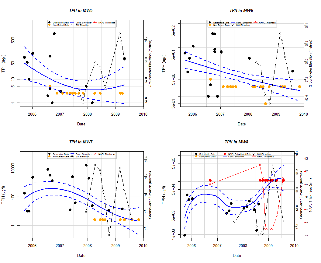
Well Trend plot:
For the investigation of historical time-series trends in solute concentrations, groundwater elevation and, if present, NAPL thickness for individual wells.
Users can overlay a nonparametric smoother which estimates the time-series trend in solute concentration.
The advantage of this nonparametric method is that the trend estimate is not constrained to be monotonic, i.e. the trend can change direction.
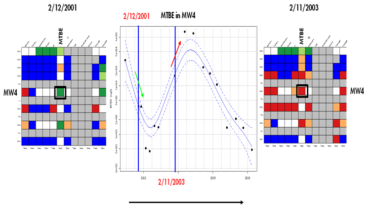
Trend and Threshold Indicator Matrix:
This feature provides a summary of the level and time series trend in solute concentrations at a particular model output interval.
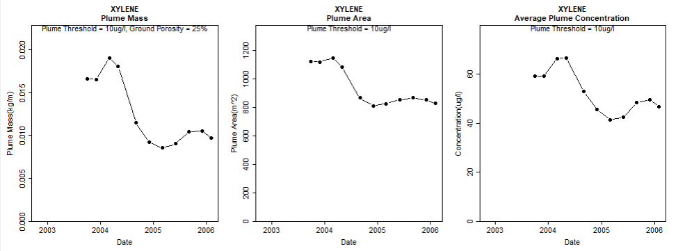
Plume diagnostics plots:
This feature enables the user to calculate and display plume diagnostic quantities (area, mass, concentration) for a delineated plume displayed with a solid red contour line.
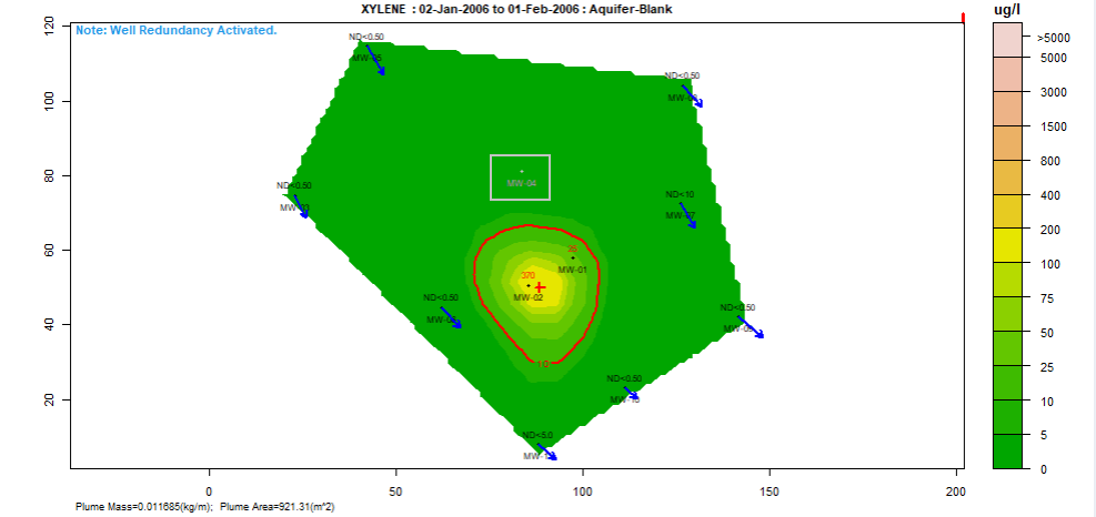
Well redundancy:
This feature enables the user to very conveniently drop a well or a combination of wells from the analysis and investigate the resultant impact.
Installation Instructions
System Requirements: Windows 8 or 10. Microsoft Office versions: 365, 2016, 2013, 2010. You need to be connected to the internet when you install GWSDAT version 3.2.
- Download and install the latest version of the open source statistical application "R" available from: http://cran.r-project.org/bin/windows/base/ . Please accept all default settings during installation. (Users must have administrator access rights to install R).
- Download the GWSDAT_v3.20.zip file from http://gwsdat.net/gwsdat_v3-20/ and unzip to somewhere on your C: Drive which is read/writable, e.g. C:\Users\A.N.Other\GWSDAT.
- Open Excel and install the GWSDAT add-in by choosing: "File" -> "Options" -> "Add-Ins" -> "Go" -> "Browse" and then select "GWSDAT V3.20.xlam" located in the "C:\Users\A.N.Other\GWSDAT_v3.20" folder. To avoid any Excel add-in security issues please ensure that this is a trusted location. See link here for troubleshooting Excel Add-in installation issues.
- A menu called "GWSDAT v3.20" will appear in the EXCEL ribbon (on right side) along the top of the EXCEL window.
Getting started
- To get started with a basic example activate menu by clicking on “GWSDAT v3.20”and then select “Open Example” > select “Basic Example" and then select "Analyse”.
- Note- the first time you run this it may take a while as it needs to download and install some additional R packages.
- To get started with a more complex example activate menu by clicking on “GWSDAT v3.20”and then select “Open Example” > select “Comprehensive Example”, and then select "Analyse”.
{multithumb}
Help and Support
Further details on GWSDAT at www.gwsdat.net
Useful Links and Presentations
GWSDAT is listed in the following ITRC guidance document: Groundwater statistics for Monitoring and Compliance
Case studies: http://gwsdat.net/case-studies/
Article: Groundwater Spatiotemporal Data Analysis Tool: Case Studies, New Features and Future Developments
Article: on benefits of spatiotemporal modelling GWSDAT in Science of Total Environment.
Article: on GWSDAT in Science Direct
Article: "Analyzing Groundwater Quality Data and Contamination Plumes with GWSDAT" in Groundwater
Supporting information for the above Groundwater article:
{multithumb}
Acknowledgements
The authors gratefully acknowledge those people who have contributed their knowledge and time to the development of GWSDAT.
The authors wish to express their gratitude to Craig Alexander, Adrian Bowman, Ludger Evers, Marnie Low, Claire Miller, Daniel Molinari and Peter Radvanyi from the department of Statistics, University of Glasgow, for their invaluable contributions to the development of the spatiotemporal algorithm.
Thanks also to Ewan Mercer from the University of Glasgow for his assistance in the development of the GWSDAT user interface.
We acknowledge and thank the R project for Statistical Computing and all its contributors without which this project would not have been possible.
A big thank you to Shell's worldwide environmental consultants for assistance in evaluating and testing the earlier versions of GWSDAT.
Thanks also to the Shell Year in Industry students who spent a great deal of time testing GWSDAT and making suggestions for improvements.
We thank both current and former colleagues including Matthew Lahvis, Jonathan Smith, George Devaull, Dan Walsh, Curtis Stanley, Marco Giannitrapani and Philip Jonathan for their support, vision and advocacy of GWSDAT.
References
-
Bowman and Azzalini, 1997. Applied Smoothing Techniques for Data Analysis: the Kernel Approach with S-Plus Illustrations. Oxford University Press, Oxford, 1997.
-
Bowman and Azzalini. sm: Smoothing methods for nonparametric regression and density estimation. R package, www.stats.gla.ac.uk/~adrian/sm
-
Eilers and Marx, 1992. Generalized Linear Models with P-Splines in Advances in GLIM and Statistical Modelling (L.Fahrmeir et al.eds.). Springer, New York.
-
Eilers and Marx, 1996. Flexible smoothing with b-splines and penalties. Statistical Science 11, 89–121.
-
Evers et al., 2015. Efficient and automatic methods for flexible regression on spatiotemporal data, with applications to groundwater monitoring, Environmetrics (open access), 26(6), 431-441.
-
Jones, et al., 2014. A software tool for the spatiotemporal analysis and reporting of groundwater monitoring data (open access), Environmental Modelling & Software, 55, 242-249.
-
Jones, et al., 2015. Analyzing Groundwater Quality Data and Contamination Plumes with GWSDAT (open access), Groundwater, 53 (4), 513-514.
- Jones, W.R., Rock, L., Wesch, A., Marzusch, E. and Low, M. (2022), Groundwater Spatiotemporal Data Analysis Tool: Case Studies, New Features and Future Developments. Groundwater Monit R, 42: 14-22. https://doi.org/10.1111/gwmr.12522
-
McLean et al., 2019, Statistical modelling of groundwater contamination monitoring data: A comparison of spatial and spatiotemporal methods, Science of The Total Environment (open access), 652, 1339-1346.
-
R Development Core Team. R: A Language and Environment for Statistical Computing. R Foundation for Statistical Computing, Vienna, Austria, 2-008. ISBN 3-900051-07-0, http://www.r-project.org